Page 35 - Mirjam-Theelen-Degradation-of-CIGS-solar-cells
P. 35
Stability of Cu(In,Ga)Se 2 Solar Cells
tion and position of molybdenum in a solar cell can be found in chapter 5. In order to
show the impact of molybdenum degradation, these layers can be divided into two
groups:
1. Stability of bare metallic molybdenum: molybdenum which is not immediately
used for further solar cell processing can be stored, but exposure of bare
molybdenum to the atmosphere can lead to a change in the electrical
properties of the later processed CIGS solar cells.
2. Long term stability of the molybdenum layer back contact in the CIGS cells.
This distinction was made since the impact of the atmosphere must be considered
for the first group (on bare metallic molybdenum). For the second group, the chemi-
cal environment of molybdenum film in a solar cell must also be taken into account,
including the presence of a thin layer of MoSe and the impact of the scribing pro-
2
cedure. More information about the impact of the scribing process can be found in
chapter 2.5.1 .
For both types of molybdenum, it was noticed that molybdenum degradation started
mainly at places in the CIGS solar cell that were damaged. This includes accidental
damages [27] as well as scratches from zinc oxide particles due to scribing and scratch -
es from sand blasting during edge preparation [28]. Since conductivity is the most im -
portant requirement for a molybdenum back contact, an overview of the degradation
(a) 10 -7 (b)
Resistivity (cm) 10 -4 Resistivity increase ( cm/h) 10 -8 -9
10
10
-11
10 -10
10 -5
Mo* Mo/MoSe 2 Mo* Mo/MoSe 2
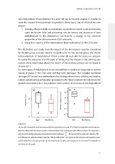
Figure 2.1
The box plots show (a) the initial resistivity and (b) the degradation rate under 85 C/85% RH of molybdenum (including mo-
o
lybdenum alloyed with aluminium or with a chromium bilayer) and molybdenum with a MoSe 2 top layer. The degradation
rates are determined by assuming a linear decrease of the resistivity ρ: ρ . The top and bottom of the box show the 25%
t
and 75% intervals, while the whiskers depict the 10% and 90% borders. The squares are the minimum and maximum values
-9
and the dashed line is the average value. The resistivity changes for MoSe 2 was negative in one case (-1x10 Ω cm/h) which is
not depicted in the graph.
33
tion and position of molybdenum in a solar cell can be found in chapter 5. In order to
show the impact of molybdenum degradation, these layers can be divided into two
groups:
1. Stability of bare metallic molybdenum: molybdenum which is not immediately
used for further solar cell processing can be stored, but exposure of bare
molybdenum to the atmosphere can lead to a change in the electrical
properties of the later processed CIGS solar cells.
2. Long term stability of the molybdenum layer back contact in the CIGS cells.
This distinction was made since the impact of the atmosphere must be considered
for the first group (on bare metallic molybdenum). For the second group, the chemi-
cal environment of molybdenum film in a solar cell must also be taken into account,
including the presence of a thin layer of MoSe and the impact of the scribing pro-
2
cedure. More information about the impact of the scribing process can be found in
chapter 2.5.1 .
For both types of molybdenum, it was noticed that molybdenum degradation started
mainly at places in the CIGS solar cell that were damaged. This includes accidental
damages [27] as well as scratches from zinc oxide particles due to scribing and scratch -
es from sand blasting during edge preparation [28]. Since conductivity is the most im -
portant requirement for a molybdenum back contact, an overview of the degradation
(a) 10 -7 (b)
Resistivity (cm) 10 -4 Resistivity increase ( cm/h) 10 -8 -9
10
10
-11
10 -10
10 -5
Mo* Mo/MoSe 2 Mo* Mo/MoSe 2
Figure 2.1
The box plots show (a) the initial resistivity and (b) the degradation rate under 85 C/85% RH of molybdenum (including mo-
o
lybdenum alloyed with aluminium or with a chromium bilayer) and molybdenum with a MoSe 2 top layer. The degradation
rates are determined by assuming a linear decrease of the resistivity ρ: ρ . The top and bottom of the box show the 25%
t
and 75% intervals, while the whiskers depict the 10% and 90% borders. The squares are the minimum and maximum values
-9
and the dashed line is the average value. The resistivity changes for MoSe 2 was negative in one case (-1x10 Ω cm/h) which is
not depicted in the graph.
33